K Nearest Neighbour
KNNs work on the principle that similar points are near each other in a feature space.
They can be used for both Classification and Regression tasks.
Definition
For an input, find the closest \(K\) examples in the training set. This is defined as the probability distribution of the label \((y)\) being the correct class \((c)\) for an input \((x)\) on some training data \((D)\):
\[p(y=c|x,D) = \frac{1}{K} \sum_{n \in N_{K}(x,D)} \mathbb{1}(y_n=c)\]where \(N_{K}(x,D)\) denotes the set of \(K\) closest training samples, and \(\mathbb{1}\) is the indicator function.
The indicator function is 1 when \(y_n\) is the same class as \(c\) so that summing over that set of \(K\) neighbors effectively count how many has the label \(c\).
We divide by \(K\) to find the fraction of neighbors with label \(c\) to get the probability that \(x\) should be labeled \(c\).
We can return this distribution or the highest label.
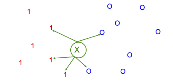
For example, for a KNN classifier for \(K=5\)

3 of the 5 have labels 1 and 2 of the 5 have labels 0.
\(p(y=1|x,D)=\frac{3}{5}\) or \((y=0|x,D)=\frac{2}{5}\)
Parameters
K Neighbors
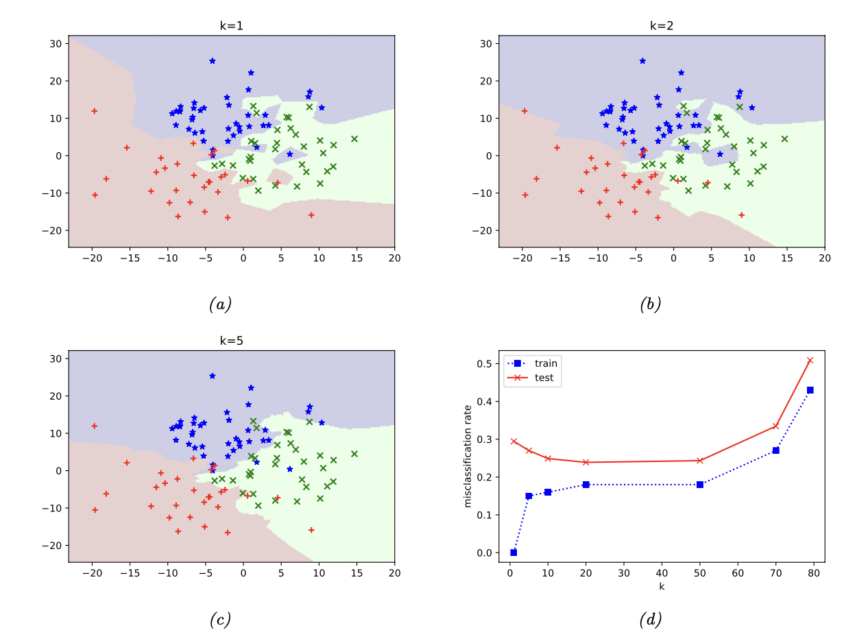
\(K=1\) is an overfit on the training set and leads to zero errors on the training set. As \(K\) increases, the decision boundaries become smoother and training error increases as we start to underfit.

Distance Metric
The most common distance metric is the Mahalanobis distance which reduces to Euclidean distance when \(M=I\) (identity matrix).
\[d_M(x,\mu) = \sqrt{(x-\mu)^T M(x-\mu)}\]If all features are on the same scale and you consider them equally important (there’s no “reshaping” or “rescaling” of the space and every dimension contributes equally), we can use Euclidean distance.
Other distance metrics include Manhattan distance, Minkowski distance, Hamming distance, and Cosine distance.
Implementation
Preprocessing
It is important to standardize the data to a common scale so that no one feature dominates the distance calculation.
from sklearn.preprocessing import StandardScaler

scaler = StandardScaler() # StandardScaler object
X = scaler.fit_transform(X) # Transform X
Finding the Right K
Too small of a K can lead to underfitting while too large of a K can lead to overfitting. We can use K fold cross validation and test values of K on the validation set to find an optimal K value.
from sklearn.model_selection import cross_val_score
from sklearn.neighbors import KNeighborsClassifier

# Perform cross-validation for different values of k
k_values = [1, 3, 5, 7, 9, 11, 13, 15, 17, 19]
cv_scores = []

for k in k_values:
    knn = KNeighborsClassifier(n_neighbors=k)
    scores = cross_val_score(knn, X_scaled, y, cv=10, scoring='accuracy')
    cv_scores.append(scores.mean())

# Find the optimal value of k
optimal_k = k_values[cv_scores.index(max(cv_scores))]
Curse of Dimensionality
KNNs do not work well with high dimensional inputs (lots of features)!
As the dimension increases, the edge length of the hyper-cube that encloses some number of data points becomes disproportionately large. In other words, the volume enclosing a set of points increases exponentially with the number of dimensions which lead to sparse distributions of data.
Neighbors far away from the original point may not be good predictors or the amount of data required to make a good prediction may be prohibitively large.
Imbalanced Dataset
KNNs rely on points from the training set to make predictions. The minority class is often sparse which can lead to misclassifications since the distance may be higher.
Performance
KNN classifiers can get within a factor of 2 of the Bayes error.
Training & Inference Complexity
KNNs store all the training data which is very wasteful in space. Finding \(K\) nearest neighbors also becomes computationally intractable as dimensionality grows.
The time complexity at inference time is O(nd) where n is the size of the training set and d is the number of features since the algorithm must compute the distance from the sample point with each point in the dataset.
References
Kevin P. Murphy. “Probabilistic Machine Learning: An introduction.” MIT Press, 2022, http://probml.github.io/book1.
https://arize.com/blog-course/knn-algorithm-k-nearest-neighbor/